Email Marketing Insights in 2025 from Neil Patel
Neil Patel recently shared powerful tips on email marketing success—think cleaner lists, smarter personalization, and value-packed content. His key message? Email isn’t dead; it’s evolving.

This is the third article in a series covering machine learning for Google Ads analysis. We are going to explore regression using multiple input features.
In the first article published on marketingland we walked through regression models you can build in excel to forecast conversions at different levels of Google Ad spend.
In the second article, we went deeper into more advanced regression models like Decision Trees & Random Forests. We detailed the advantages & disadvantages of these complex models.
Previously we used only one variable, ‘cost per day’ to try and predict the number of ‘conversions per day’ within a Google Ads account. In this article we will go deeper still and see what happens when we use multiple variables beyond just ‘cost’ to make predictions. Can we make better predictions with more input features?
You can find the python code here as a worked example
There are many different metrics in a Google Ads account that contribute to performance. Cost, time of day when the click occured, mobile device used, click through rate on ads, etc… How do we know which features are the best predictors of conversions?
Random Forest models are very transparent and allow us to see which factors influenced their decision making. In his fantastic course on machine learning, Jeremy Howard of fastai.com recommends building a quick random forest with all feature inputs to find features of high importance. We can then eliminate low importance features and drill down into the remaining features.
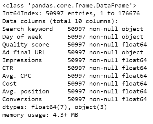
The first step is to export the data from the Google Ads report editor & bring it into a python supported notebook like jupyter notebook. We imported 9 features from Google Ads, 6 of them numerical (floats) and 3 categorical (objects). Our dependent variable (what we were looking to predict) is Conversions. Our Dataframe had 50,997 rows of data after we removed rows with missing values & rows with 0 clicks. Below is a summary of the dataframe after initial preprocessing:

After importing the data and cleaning it up, we split the data into a training set (80%) and a holdout test set (20%). We trained a random forest (RF) model on the training set. With then used the holdout set to test the predictions from our model. As an indicator of performance, we found the Root Mean Squared Error (RMSE) was 1.42.
For comparison, if we were to take the mean value of all conversions in the training set & use that to predict the conversions in the holdout set, the RMSE of predictions against actuals would have been 2.9. So the RF model had less error and was a better predictor than predicting just the average.
The following were the most important features used by the RF in predicting ‘Conversions per day’ :

We can see that ‘Cost’ was clearly the strongest feature. This was followed, not so closely by other features like ‘Impressions’ & ‘CTR’.
If we run a new random forest model on this dataset, this time just using only ‘Cost’ & no other features, the RMSE is 2.06. This is a significantly higher error than the previous model which uses all 9 features. But it is still better then just predicting the average.
Also, if we were to run a simple linear regression (LR) between cost & conversions, the RMSE turns out to be 2.02, which is very similar to the result achieved by the Random Forest based on only ‘Cost’.
To summarise, we achieved the following RMSE’s on our holdout set with our predictions:
We can see the difference between the RF & the linear models more easily when we visualise them. The orange line is the linear model, the pink the random forest:

Why is cost such an important predictor in Google Ads? Simply put, the more you spend, the more traffic you generate and the more leads come through. Other factors, like the average position of ads hold some importance, but the daily spend influences everything else.
There are a number of limitations to consider. Firstly it’s difficult to export from Google Ads report editor a large number of features. Features in Google Ads are classified as metrics & dimensions. Some metrics cannot be displayed with some features, so we can only export some combinations. This makes it difficult to truly analyse which feature combinations are best predictors. There are more to explore
Also consider that the dataset we used was not huge. It contained less than 60,000 observations (rows). We could increase the number of observations by pulling data from further back in time. However, the more recent the data the better, since it will more accurately predict what will happen in the near future. So it’s not ideal to go to far back either.
In summary – more columns (features) and more rows (observations) will help the model generate more accurate results.
I recommend try running a random forest on a different set of feature columns. There are many feature combinations which one could try.

Neil Patel recently shared powerful tips on email marketing success—think cleaner lists, smarter personalization, and value-packed content. His key message? Email isn’t dead; it’s evolving.

SEO copywriting: user-focused, keyword-rich content. Optimize URLs, titles, and meta descriptions. Balance search engines and audience needs to boost rankings and drive traffic.

Brand owners can control their Amazon listings and remove unauthorized sellers by enrolling in Brand Registry. This grants priority in content updates, access to A+ content, and tools like Brand Transparency and Project Zero.
Subscribe to receive exclusive industry
insights & updates
Copyright © 2014 – 2025 One Egg. All rights reserved.
Subscribe to receive exclusive industry insights & updates